AI applied to football: uncover the most promising talent
Clustering algorithms on football players
Since Data Science democratisation, Clustering (also called Data Partitioning) has been one of the most recurrent challenges in this field.
Clustering techniques consist in applying Machine Learning algorithms to heterogeneous groups of data, in order to divide them into subsets (clusters) where data points have similar values and characteristics. These homogeneous clusters can then be analysed in order to identify and understand their behaviour within their group. The fields of application of Clustering are unlimited: Financial Analysis, Marketing, Demography, etc.
Introduction
During this time of the year, which is synonymous with the winter mercato, football players are evaluated and valued according to various attributes such as their age, their efficiency in front of goal, their vision of the game or even their technical and physical characteristics.
Through an educational and playful approach, the purpose of this article is three-fold. First off, Clustering methodologies will be applied to football players data in 2016. Secondly, resulting clusters will be used to forecast 2020 data, and the most likely player transfers will be identified during this period. Finally, players with a strong financial potential will be exposed at the end of this article.
USED DATA
Datasets used in the present article derive from FIFA’s videogames 2016 and 2020 releases. They result from a general volunteering evaluation process made by many passionate advocates of Football, as well as actors having evolved professionally in this domain. Data has been harmonised in order to avoid inconsistencies and to account for differences in the number of reviewers by championship, clubs and players, with the idea to describe as accurately as possible the world of Football at a precise moment.
Step 1: Data Collection
The first step is to acquire all the necessary tools to carry out the clustering described above. Python and Jupyter Notebook were selected as the programming language and development environment in this analysis; sklearn, numpy and pandas were our most powerful weapons in terms of required libraries.
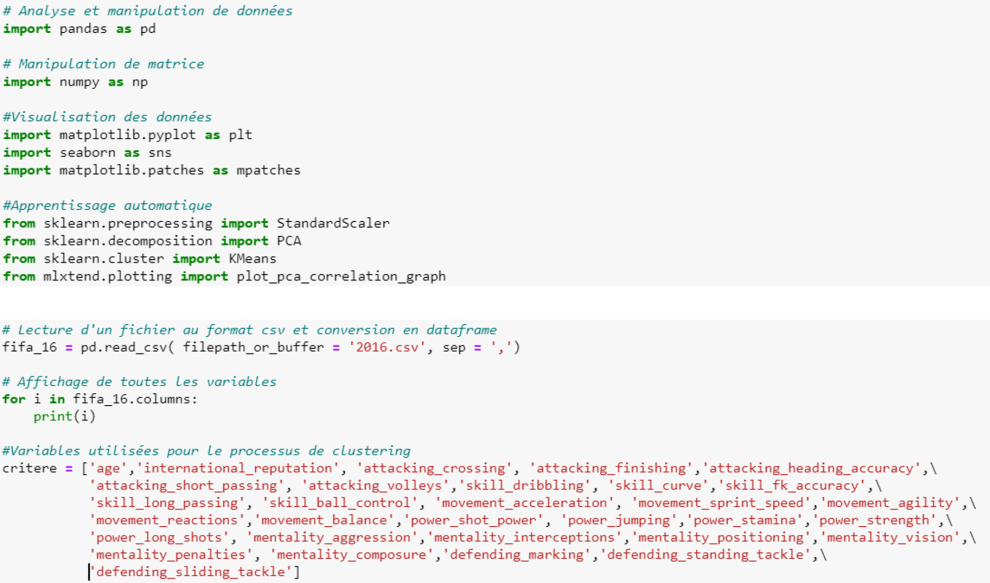
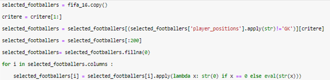
Data sample was composed of the 200 best rated players in FIFA 2016. Indeed, we acknowledged that the latter were less prone to poor data quality due to a focus of evaluators on these best players and clubs. Goalkeepers were excluded from this analysis because of their unique role in the game.
Most variables used in this analysis were presented as a character sequence in the form of “x+k”, where x is an integer and k a relative integer. x corresponds to the rating given to a player in his last performance, while k represents an adjustment made to this rating. If players had great performances, then k is positive (k > 0), and conversely, if players had bad performances, then k is negative (k < 0). We then apply an eval function to our variables allowing us to parse our character sequence arguments and evaluate them as a Python expression. In this way, eval(80+2) is replaced by 82.
Step 2: Dimensionality Reduction (Data Pre-processing)
Some of the variables are defined on different references, which makes them difficult to compare with each other. To overcome this constraint, an affine transformation called Centering and Reduction is applied. It consists in imputing the mean of all the variables studied and dividing the result by their standard deviation. This transformation allows to generate variables with zero mean and unit standard deviation, while keeping correlation properties between them.
Moreover, Clustering algorithms, presented in the next part, depend on the proximity between each individual studied. Arbitrarily, this proximity is measured using the Euclidean distance. Indeed, widely used, the Euclidean distance is considered one of the most intuitive measurements. However, the Euclidean distance loses all its meaning in high-dimensional spaces, i.e. having too many variables.
It is therefore of great importance to first perform a dimensionality reduction technique, such as Principal Component Analysis (PCA) [3]. The latter consists in transforming a high-dimensional dataset of correlated variables into a reduced dataset of new variables that are decorrelated from each other, while keeping as much of the variability in the data as possible. However, it is important to state that this technique leads to a loss of information.
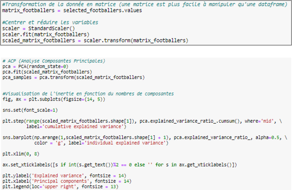
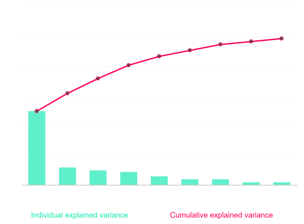
Once the PCA has been completed, it is therefore necessary to decide on the number of components. A new problem appears: maximizing the information absorbed by the components, while at the same time minimizing the number of components to be embedded, and keep low dimensionality. Naturally, it is therefore necessary to keep components that have absorbed most of the information, such as the main components 1, 2, 3 and 4. These can be observed in the bar chart below, each absorbing 48%, 12.1%, 9.5% and 8% of information respectively. In order to stay within a perceptible space, the first three components were chosen, and together they absorb nearly 70% of the information.
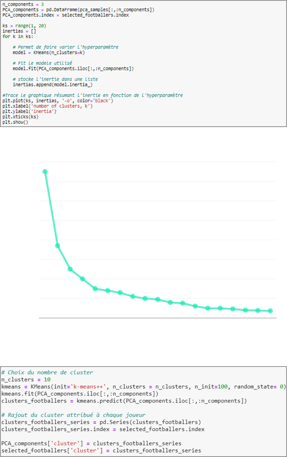
Step 3: K-means Algorithm (Modeling and Visualization)
Now that the new dataset includes only principal components, applying a Clustering algorithm is now plausible, and a K-means algorithm has been chosen [4]. It is able to group individuals in the dataset into K distinct homogeneous groups. Thus, players with similar characteristics will be located in the same cluster. Note that a football player can only belong to one and only one cluster.
Parameter K is to be defined, raising the following issue: Finding a K that sufficiently minimizes the variance within a cluster. In the same way as principal components were chosen, the cardinality of K should be increased as long as the addition of a cluster significantly reduces the inertia present in the entire dataset. This method is called the "Elbow Method". Other methods exist to determine the optimal K: Hierarchical Ascendant Classification, etc. Results indicate that from the 10th cluster onwards, the inertia almost no longer decreases. Thus, the number of clusters chosen is 10.
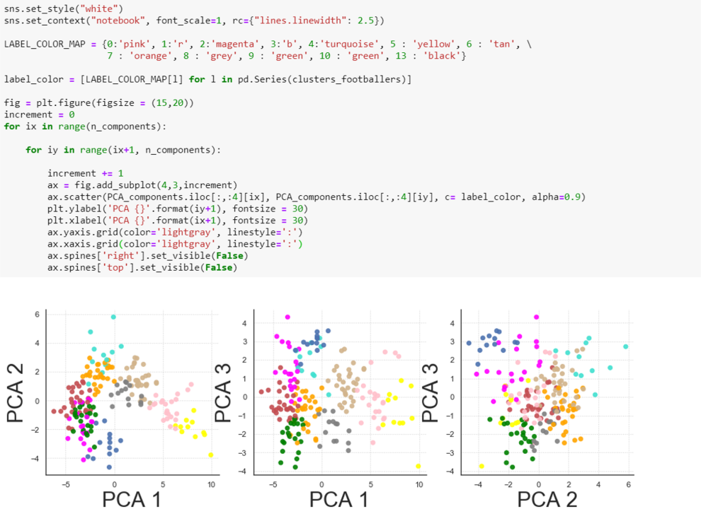
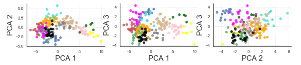
Since data are now projected in a three-dimensional space, it is possible to visualize the clusters in three different planes, each composed of distinct pairs of principal components. The use of a three-dimensional figure can lead to a loss of information, because it depends on the angle of perception; it is then preferable to propose several planes in two dimensions.
Step 4: Clustering Results On FIFA 2016 data
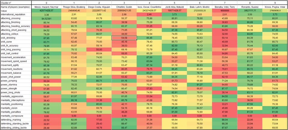
Ten clusters have been generated, each one reflecting the skills and level of the players in 2016. The heatmap above summarizes in a macroscopic way the content of these clusters. An average score for each variable is calculated to highlight the discriminating features of each one of them. The green and red colors respectively mean that all the players in a cluster have either a high or a low level of a specific characteristic, while a yellow coloring reveals an average level. It is observed that players playing in the same game registers are grouped together, confirming that clusters were correctly constructed.
Cluster 0, red color: this cluster absorbed versatile offensive players, able to evolve at all attacking positions. According to results, these are players that dominate ball control, and possess an ability to dribble and to eliminate a player while being great at shooting free kicks.
Cluster 1, dull beige color : players in this cluster are considered to be defensive technical profiles. According to FIFA 16 data, these are players that have a very good sense of anticipation.
Cluster 2, blue color: this cluster regroups natural goalscorers. These are players who position themselves in the right place in order to be in the best conditions to act.
Cluster 3, pink color: in addition to cluster 1 (dull beige, defenders), cluster 3 also includes defenders. The distinction is made by the fact that players in this cluster are particularly proficient in the aerial game but less skilled during other game phases. This can be easily visualized on the heatmap, which reveals that many of the qualities are tending towards orange.
Cluster 4, green color: this cluster includes players having typical qualities of game leaders. They are characterized by an ability to accelerate, to keep the ball, and they have a certain liveliness when they have to make a decision.
Cluster 5, grey color: Side back players are located in this data partition. It is interesting to note that Matuidi, who is a midfielder, has characteristics similar to those of Jordi Alba and Dani Alves according to FIFA 16 data.
Cluster 6, orange color: this cluster is represented by the versatile midfield players. No attribute tends towards a reddish complexion.
Cluster 7, color yellow: this cluster gathers physical defenders having a "warrior's mentality", as evidenced by a high score on variables mentality_agression and power_strength.
Cluster 8, magenta color: great attackers are gathered in this cluster. According to the data, these players excel in making goals and in the last pass. Finally, this cluster is close to cluster 0 (red, versatile attackers), with the only difference that cluster 8 players appear to have a higher taste for goals.
Cluster 9, turquoise color: according to results, midfielders are concentrated in this cluster. These players are characterized by an ability to project themselves forward in order to get closer to the goal, but also by having a high score on dead-ball positions, good ball striking and excellent vision of the game.
Step 5 : 2016 vs. 2020
As explained at the beginning of this article, the purpose at this point is to identify inter-cluster transfers between 2016 and 2020, in order to list players having high added value. After projecting 2020 data through the main components constructed with 2016 data, some transfer channels were revealed.
The table below represents inter-cluster transfers carried out between 2016 and 2020.
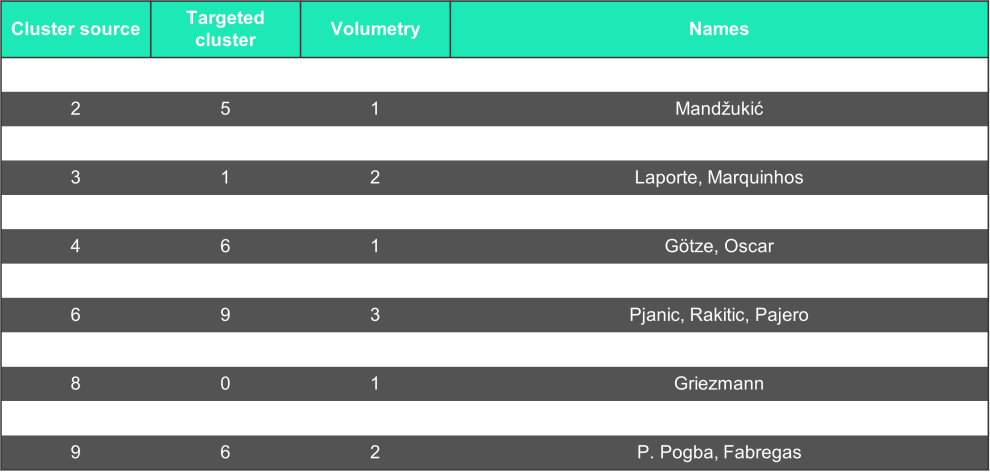
According to the heatmap, clusters 0 and 8 group players with the best market value. It can be interesting for a club wanting to trade players to understand how clusters are fed over time. Transfer channels feeding clusters 0 and 8 are:
- Cluster 2 powers Cluster 8 when natural goalscorers change their way of playing in order to participate more in the construction of the game. This transformation is usually done when a player's career is coming to an end.
- Cluster 4 feeds cluster 0 when offensive midfielders reach a sufficient level of skills allowing them to score a lot of goals.
- Cluster 6, when versatile players change to a position closer to the goal on the field.
- Cluster 0 and 8 are self-powered.
Thus, in order to generate profitability, clubs have every interest in recruiting young players belonging to clusters 4 or 6 (green and orange colors). Indeed, targeting young players is highly relevant because of their large margin of progression.
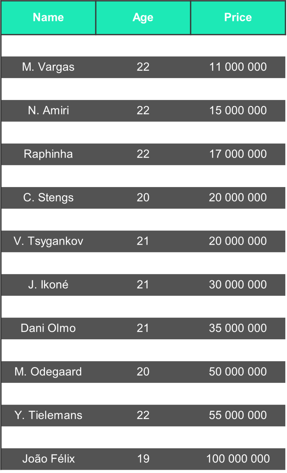
After filtering players and keeping only those who are under the age of 23, a projection of the main components and a list of players who have or are likely to develop a high market value is presented next:
Conclusion
Thanks to Clustering techniques, through the present tutorial we have been able to perform a descriptive analysis of the data. The latter allowed us then to study inter-cluster exchange channels. Finally, from the exploitation of these channels we have derived a list of players able to provide high profitability. Raphinha, already bought by Rennes for 21 million euros in the summer of 2019 when he was only worth 8 million euros at the time, is a serious candidate according to our results. Re-evaluated recently in January 2020 at 17 million euros, his price has doubled. In view of the 2019-2020 season, it is possible that his qualities will begin to slide towards those of clusters 0 or 8, and potentially that at the same time his price will increase.
Sources
[1]https://www.kaggle.com/stefanoleone992/fifa-20-complete-player-dataset
[2]https://mcetv.fr/mon-mag-culture/mon-mag-gamers-time/fifa-18-calcul-notes-joueurs-2809/
[3]https://scikit-learn.org/stable/modules/generated/sklearn.decomposition.PCA.html
[4]https://scikit-learn.org/stable/modules/generated/sklearn.cluster.KMeans.html