How to avoid GDPR issues using GAN (Generative Adversarial Networks)
With Big Data development, we have seen in those last decades the emergence of many issues raised by the massive use of data. In particular, personal data protection issues are pervasive for companies that store their customers’ data.
With Big Data development, we have seen in those last decades the emergence of many issues raised by the massive use of data. In particular, personal data protection issues are pervasive for companies that store their customers’ data. In Europe, these issues are framed by the GDPR law (General Data Protection Regulation) which was established in 2016. This law requires a considerable effort from companies to supervise and justify the provision of data according to their sensitivity. This slows down the data exploitation processes, for example in the use of data to build machine learning algorithms. One way to solve this problem could be to generate a fictive dataset from the original one and then use and share this dataset. The goal of this new dataset is to be non-sensitive but to keep all the characteristics of the old dataset so we could build efficient algorithms based on it. In this article, we will see how and to what extent this is possible with a GAN algorithm.
What is a GAN (Generative Adversarial Networks)
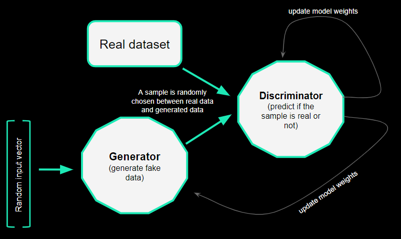
GAN stands for Generative Adversarial Networks. They are notably the algorithms used to generate fake images or videos: it is what is commonly called deepfake. The general principle of this algorithm is to train two models (neural networks) that will compete. The first model is a generator: its goal is to generate data very similar to the dataset we want to replicate. The second model is a discriminator: its goal is to identify whether a sample of data is real or generated.
The discriminator will randomly be fed either by fake data created by the generator or by a sample from the real dataset. If the discriminator classifies the sample well, it means the generator didn’t manage to fool it. The loss values of the discriminator and the generator will then be affected positively and negatively respectively. Thus the weights of the neural network models will be affected accordingly. If the discriminator is wrong in its prediction, the opposite effects occur.
GAN algorithm principle
We used for our study a library that allows us to easily train and use GAN , but if you want to know more about how to create GAN yourself, you can follow this PyTorch tutorial.
The particularity of our study
In this article, we will see step by step how to use GAN to generate tabular data. When for deepfake, GAN were used to generate triplets of integers (photos or videos), here the type of data we will generate is broader: numeric, strings, class fields, dates, etc..
We will check how to generate such various data thanks to CTGAN (Conditional Tabular GAN) models from sdv library and then compare the original and the generated dataset on the following topics:
- Distribution through class fields, or quantitative fields,
- Correlations between quantitative fields,
- Quality of the dataset (outliers, NaN values, duplicates …),
- Sensitivity of the data (GDPR fields).
Studied Datasets
We will generate data from 2 different datasets :
The first one was created with samples of white and red wine from Portugal. It has 2 class fields: type of wine (white or red) and quality (0 to 10); and 11 continuous quantitative fields (alcohol content, acidity, residual sugar, etc.). For more details about this dataset, consult the reference [Cortez et al., 2009] [4].You can download it here.
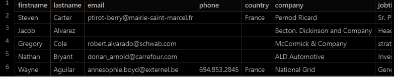
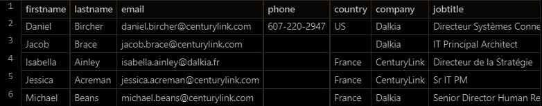
For the second one, we chose a dataset representative of a customer database, with various types of fields: categorical fields (country, company), discrete string fields, (email, name, phone number), date (createdate). This dataset has interesting data quality properties that we will study in further parts. Here is an extract :
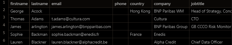
As training sdv CTGAN requires many GPU resources, we only trained GAN on the 1000 first rows of this dataset (ordered by lastname) during our study.
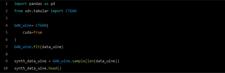
First steps with CTGAN
Let’s see how simply we can train and use a CTGAN (Tabular GAN) model thanks to the library sdv.tabular. We will here create a dataset of the length of the real dataset.
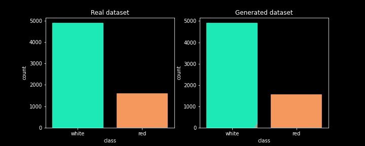
Once the dataset is generated, we can first check that the distribution on a classification field of the synthesised dataset matches the distribution of the real dataset!
Distribution of type of wine for Real & Generated Dataset
Let’s now study further the similarity between those two datasets.
Correlations & similarity study:
Correlations between numeric fields
To better understand how well the generated dataset fits the real one, the idea is now to compare the correlations between quantitative fields. For example, we can draw two scatterplots to study the correlation differences between the pH and fixed acidity fields (which should be correlated).
Correlation between pH and fixed acidity for Real & Generated Dataset
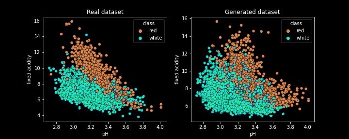
Two interesting things to notice from this graph :
- The generated dataset is not a simple replica of the original dataset: new values are created,
- The correlations between those two fields seem quite well replicated on the generated dataset (but not perfectly).
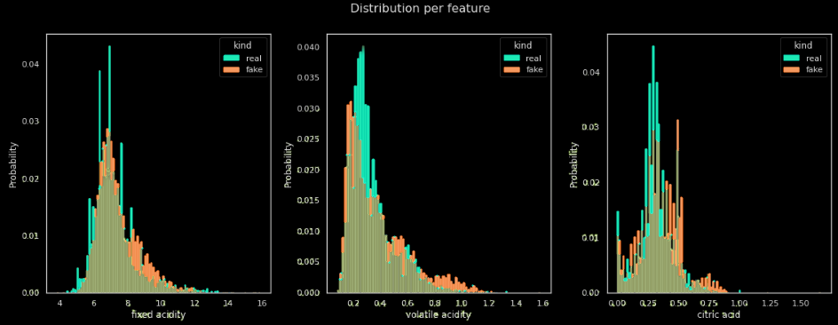
More generally, it would be interesting to conduct this study on all numeric fields and display it on a grid of graphs: python library table_evaluator is very convenient to compare 2 datasets. Below is the code and some interesting resulting graphs.

Comparison of distribution on some numeric fields
Correlation matrix on real dataset, generated dataset & differences
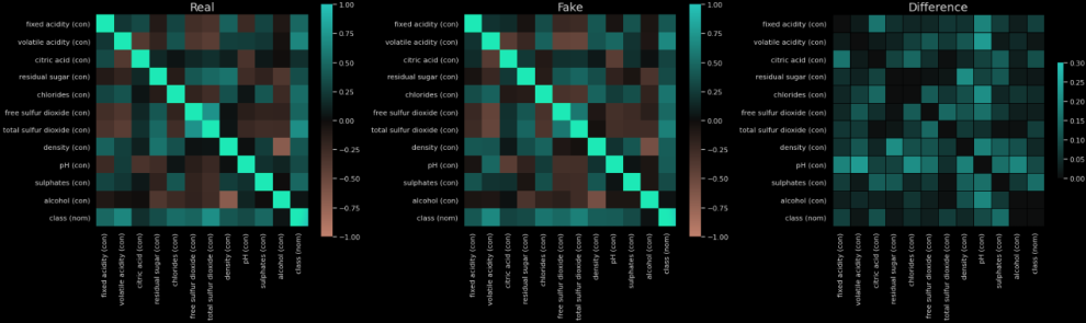
Among other graphs, this library plots distribution graphs on all numeric fields and correlations matrices. Those graphs allow us to easily identify the gaps in our generated dataset. For example, we can see on the Difference graph that the correlation between the volatile acidity and the pH is quite badly replicated on the synthesized dataset (difference of correlation of about 0.30).
This matrix of correlation differences shows us a way to create a similarity score by calculating the average of those differences. However, this metric makes sense only if there are indeed correlations in the original dataset; otherwise, any dummy dataset could have a very good similarity score to the real one.
Metrics of performance integrated into the sdv library
The sdv library directly provides us with an interesting module to compare two datasets on different metrics. It computes some basic statistical models on the datasets, below is the code.

Similarity metrics & scores between synthesized and real dataset
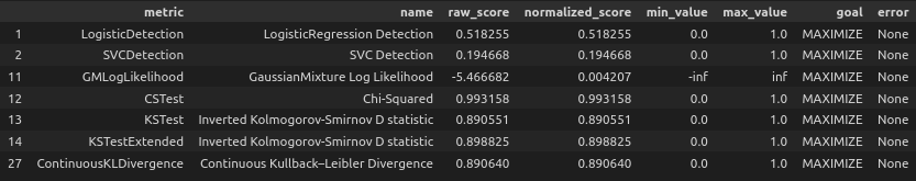
We thus obtain scores such as ChiScore, LogisticDetection score among other scores which are calculated on numerical fields.
SDV also allows us to easily analyse how a classification model, trained on the synthesized dataset, behaves on the real dataset.

Typically, a Binary Decision Tree Classifier trained on the synthesized dataset predicts with an average accuracy of 0,95 the type of wine of the real dataset. As a comparison, a decision tree classifier trained on the real dataset predicts with an average accuracy of 0,98 the type of wine of a real test dataset.
Data Quality Comparison between Original & Generated Dataset
We will now focus on a different property of datasets: their “quality”. To analyse the quality differences between the real and the generated dataset, we will focus on 3 main properties:
- Outliers
- NaN values (fields that are not filled)
- Duplicates
Outliers :
We will check how the model reacts when we add some outliers to the training dataset. We thus decided to randomly add 15 samples of wine with an unusual pH value (around 7). Here are the differences between the spoiled dataset, the dataset generated by a model trained on clean data, and the dataset generated by a model trained on data with outliers.
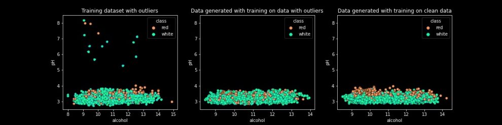
We can notice on the middle graph that no outliers are generated by the model when it’s trained on data with outliers.
To check the effects of the outliers on the GAN trained on them, we computed the accuracy of a Decision Tree model trained on data generated by this GAN to predict the type of wine of real samples. Once again, we obtained an average accuracy of 0,95.
As a conclusion of our tests on outliers: training a GAN on data with outliers did not allow us to obtain outliers in the generated data. On the other hand, this doesn’t seem to have degraded the model either.
From now on, we will use the second dataset with personal data (name, email, company, etc.). This dataset, similar to many tables in companies’ databases, contains quality deficiencies and in particular null values and duplicates.
Firstly, here is an extract of a dataset generated by a CTGAN trained with default parameters :
Dataset generated by a GAN trained with default parameters
At first sight, we can already notice that correlations between the fields firstname, lastname and email seem to have disappeared. Let’s now compare the properties of this dataset and the original one on quantitative metrics.
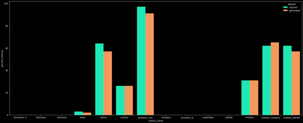
Null values:
To study how a CTGAN generates a dataset similar to the real one in terms of NaN values, we firstly compared the proportion of NaN values by field between the real dataset and the real one.
The below graph shows that CTGAN generates NaN values approximately in the same proportions as the real dataset.
Percentage of missing values by column for the original and generated datasets
To push further the investigation, we then studied how the correlations of NaN values between the fields are replicated by the model.
Comparison of correlations of NaN values between real & generated dataset
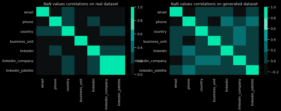
The correlation matrix of the real dataset (left graph) doesn’t show particular correlations except for the fields linkedin_company & linkedin_jobtitle. Their NaN values are fully correlated: if one of the two fields is filled, the other one will also be. However, for the generated dataset, this correlation doesn’t appear.
As another example, a small study showed that there is no logical link between the countries and the format of phone numbers on the synthesized dataset.
More broadly, we can here intuit that by default, a basic sdv CTGAN model doesn’t create any correlations between a discrete string field and another field.
Duplicates :
Let’s study if a basic GAN produces datasets with duplicates to the same extent as the real dataset. To compare the number of duplicates generated, we used the module Data Deduplication of the tool Smart Data Quality (SDQ). SDQ is a tool to accelerate data quality analysis and processes through different modules: Data Deduplication, Data Enrichment, Quality Diagnoses & Data Normalization. To know more about it, don’t hesitate to read the article “How SmartDataQuality.ai accelerates a company’s data quality process”.
The Data Deduplication module automatically detects duplicates. It is mainly based on the Levenshtein distance which allows us to compute a smart score comparison between two strings. This distance is computed between each field of each pair of rows so that we finally obtain the most probable duplicates of the dataset with an accuracy score.
By selecting specific columns (name, firstname, email, phone number, company name, jobtitle & country), and fixing a confidence score threshold of 85%, SDQ finds out 13 duplicates among the 1000 studied rows of the real dataset (1,3%).
Result Screen of the deduplication module of the tool Smart Data Quality
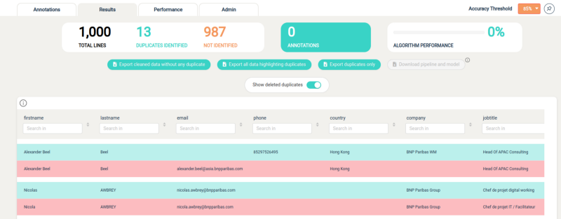
By doing the same study on the synthesized dataset, SDQ doesn’t find any duplicates.
This phenomenon can once again be explained as the model doesn’t automatically keep correlations between string fields. Indeed, we already noticed that firstname, last name & email are not correlated at all in the synthesized dataset as opposed to the true dataset.
CTGAN to create GDPR compliant datasets
We will in this final part study whether GAN can help us to generate a GDPR-compliant dataset.
Our goal is to create a model that can be applied to any dataset to add noise to sensitive fields and anonymize personal data (email, phone number, etc.). After running the model, we want to obtain a dataset that is no longer governed by GDPR laws, so that it can be shared and used without all the time-consuming associated processes.
This is why we will now focus on the generation of discrete string fields (email, phone number, IBAN, etc.) as they contain the sensitive & PII (Personally Identifiable Information) data.
Default generation of discrete string fields by the sdv CTGAN :
At this stage, let’s have a look at the string fields generated by the CTGAN, below is a sample.
By running the following small script we noticed that 100% of the string data of the generated dataset was taken from the original one. This means that there is no new data created.

As we don’t want real data for these fields, an idea is to use the faker library during the creation of the dataset.
Faker Providers in CTGAN:
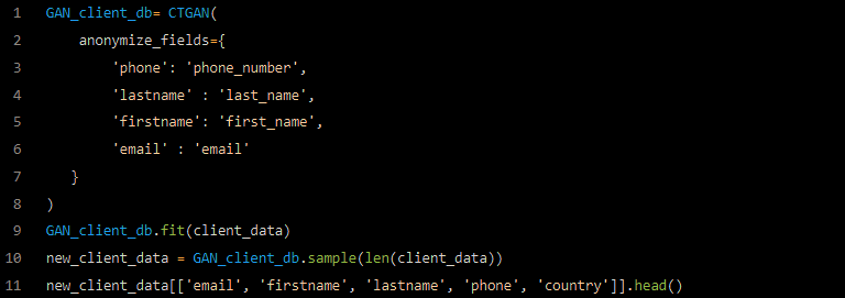
SDV gives us the possibility to use faker providers for many type of data (here is the link with the list of all providers available). Below is the code to parameterize the CTGAN model to implement these providers for each sensitive field we want to anonymize.
And here is what the generated data created looks like:
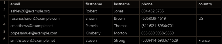
We thus managed to create a dataset without PII data, however, we can note that:
- There are no correlations between first_name, last_name & email,
- The fields are always filled in; the proportions of NaN values of the generated dataset do not fit the ones of the true dataset anymore,
- The phone number format does not match the country.
How to anonymize fields & keeping dataset properties :
SDV also allows us to set constraints for the CTGAN models. We could for example force the model to create the email field as a concatenation of the firstname, lastname, and company domain. However this feature only works if the constraint is always fulfilled in the training dataset (which isn’t true).
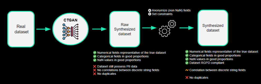
This lack of flexibility finally encourages us to create our own data processing algorithm which fits our needs. We thus propose the following steps:
1- We train and use a CTGAN with default parameters to generate a new dataset,
2- We then use the faker library to anonymize sensible fields, but we let the NaN values to NaN as CTGAN generated them with the right proportions compared to the original dataset,
3- For some fields such as phone number, we can set a rule to fake it with the country-specific format
4- We update the columns that can be set determined from other ones (email for example can be determined from faked firstname, lastname & company fields).
Conclusion:
Through this step-by-step study, we were able to understand the benefits of using GAN, especially to reproduce correlations between categorical or numeric fields. By using GAN on a dataset with many discrete free fields, we saw interesting properties as for example the reproduction of proportions of NaN values, however, we also encountered the limitations of these models, especially for creating new strings.
To circumvent this we then proposed a simple data processing pipeline that would use a faker library and compute scripts to set some specific constraints. This solution still has some weaknesses such as the creation of duplicates which is for now impossible, but the main objectives are fulfilled ! By running this model, we are able to transform a dataset so that it becomes neither sensitive nor subject to GDPR regulations. The replicated dataset is therefore shareable without any risk or special process, and can be used for studies as it replicates most of the original dataset properties.
Links & References
- PyTorch DGAN tutorial
- SDV Librairy, CTGAN — Model https://sdv.dev/SDV/user_guides/single_table/ctgan.html
- Cortez et al., 2009 — Modelling wine preferences by data mining from physicochemical properties